Generalizable Multi‑Agent Planning from Signal Temporal Logic Specifications via Diffusion

Joe Eappen, Zikang Xiong, Shreyash S. Iyengar, and Suresh Jagannathan

Purdue University

3‑Minute Overview

Abstract

Multi-agent systems in the real-world (e.g., drone swarms, autonomous cars, warehouse robots) must satisfy rich, temporal tasks while avoiding collisions. Signal Temporal Logic (STL) elegantly encodes such objectives, but current STL planning methods face critical limitations. State-of-the-art optimization-based approaches can handle arbitrary STL specifications but struggle with scalability, becoming computationally impractical as the number of agents grows. Learning-based methods efficiently handle a large number of agents with rapid planning times but fare poorly when deployment-time objectives differ from those used during training, and do not support planning tasks that require different specifications to be ascribed to different agents (i.e., heterogeneity). This fundamental trade-off between generalizability and scalability presents a significant challenge for realizing multi-agent STL planning algorithms in practice. To overcome this challenge, we introduce a new diffusion method for multi-agent planning with STL specifications. Using a differentiable approximation of STL, we integrate the STL gradient in the denoising process, making our approach generalizable to novel formulas constructed from a fixed set of predicates available at evaluation, while achieving the same scalability as existing learning-based methods. Our method supports heterogeneous specifications, and by using diffusion models, naturally enhances plan diversity, thereby significantly reducing safety-related violations (e.g., collisions) among agents. A detailed evaluation study justifies the utility of STL-guided diffusion-based multi-agent planners for constructing generalizable, scalable, and diverse plans.

Diffusion Process visualized for N=8 agents with heterogeneous tasks

Diffusion Process visualized for N=32 agents with heterogeneous tasks

Real‑World Demonstration

Heterogeneous sequence demo with 3 goals on N=10 robots in the Robotarium testbench.

Diversity Videos

Note: These clips illustrate qualitative diversity across rollouts for the sequence specification for 3 goals with all agents following the same task (Homogeneous).

Diffusion

GNN-ODE

STLPY

N = number of agents; Spec abbreviations: Seq. = Sequence.

Diversity Metrics

How the metrics are computed

Notation. We consider valid trajectories as polylines $\tau_{s_i}=\{\mathbf{x}^{(i)}_t\}_{t=0}^{T-1}\subset\mathbb{R}^2$ for $M$ successful agents over $T$ steps.

Path Overlap (↓)

Occupancy grid. Overlay a uniform grid of resolution $r_{\text{grid}}=0.3\,\mathrm{m}$ on the workspace $[x_{\min},x_{\max}]\times[y_{\min},y_{\max}]$ (e.g., $x_{\max}=y_{\max}=6$, $x_{\min}=y_{\min}=-0.5$). For agent $i$, the binary occupancy mask is \[ O^{(i)}_{u,v}=\mathbf{1}\!\left[(u,v)\in \text{cells}\bigl(\tau_{s_i}\bigr)\right]. \] The (normalised) overlap among $M$ agents is \[ \text{Overlap} \;=\; \frac{\displaystyle\sum_{u,v}\Bigl(\bigwedge_{i=1}^{M}O^{(i)}_{u,v}\Bigr)} {\displaystyle\sum_{u,v}\Bigl(\bigvee_{i=1}^{M}O^{(i)}_{u,v}\Bigr) + \varepsilon}, \qquad \varepsilon=10^{-6}, \] where $\wedge$/$\vee$ denote logical AND/OR over agents. $\text{Overlap}\!\approx\!1$ means identical footprints; $\approx\!0$ means disjoint footprints.

Path Entropy (↑)

From $O^{(i)}_{u,v}$ build the cumulative grid \[ \mathrm{occ}_{u,v}=\sum_{i=1}^{M}\sum_{t=0}^{T-1}\mathbf{1}\!\left[(u,v)\in \text{cell}(\mathbf{x}^{(i)}_t)\right], \] and the visited set $\mathcal V=\{(u,v)\mid \mathrm{occ}_{u,v}>0\}$ with $V=|\mathcal V|$. Define \[ p_{u,v}=\frac{\mathrm{occ}_{u,v}}{\sum_{(a,b)\in\mathcal V}\mathrm{occ}_{a,b}},\quad (u,v)\in\mathcal V, \] and report the normalised Shannon entropy \[ \hat H \;=\; -\frac{1}{\log V}\sum_{(u,v)\in\mathcal V} p_{u,v}\log p_{u,v}. \]

Pairwise Distance & Cluster Statistics

Distances. For each pair $(i,j)$, compute the discrete Fréchet distance $D_{ij}=d_F\!\bigl(\tau_{s_i},\tau_{s_j}\bigr)$, forming a symmetric matrix $D\in\mathbb{R}^{M\times M}$. The mean pairwise distance (reported as “Mean Pairwise Dist. (↑)”) is \[ \overline{D} \;=\; \frac{1}{M^2}\sum_{i=1}^{M}\sum_{j=1}^{M} D_{ij}, \] where higher values indicate more separation among successful plans.

Graph & clusters. Build an undirected graph $G=(V,E)$ with $V=\{1,\ldots,M\}$ and \[ (i,j)\in E \;\Longleftrightarrow\; 0 < D_{ij}\le \Delta\tau,\quad \Delta\tau = 1\,\mathrm{m}. \] Let $\text{ConnComp}(G)$ be the connected components, $k=|\text{ConnComp}(G)|$, and $C_c$ a component. We report:

  • Num. Clusters (↑): $k$ (larger $\Rightarrow$ more distinct route groups).
  • Max Cluster Fraction (↓): $\displaystyle\max_c |C_c|/M$ (smaller $\Rightarrow$ no single dominant route).
  • Agents per Cluster (↓): $\displaystyle \frac{1}{k}\sum_c |C_c|$ (smaller $\Rightarrow$ more evenly split).

Legend: “↑” higher is better; “↓” lower is better. These metrics complement success/safety to characterise diversity.

All diversity metrics for $N=16, 32$ agents in the Homogeneous task setting. D-MA: Diffusion-based Multi-Agent (Ours), G-O: GNN-ODE planner, STLPY: MILP planner. Best results are in bold.
Spec N Agents per Cluster (↓) Max Cluster Fraction (↓) Mean Pairwise Dist. (↑) Num Clusters (↑) Path Entropy (↑) Path Overlap (↓)
D-MAG-OSTLPY D-MAG-OSTLPY D-MAG-OSTLPY D-MAG-OSTLPY D-MAG-OSTLPY D-MAG-OSTLPY
Branch 16 1.093.812.35 0.120.560.33 2.632.102.33 14.674.206.80 0.930.880.93 0.000.080.00
32 1.036.584.10 0.040.790.20 3.432.352.35 31.104.877.80 0.900.860.92 0.000.000.00
Cover 16 1.086.403.02 0.120.810.47 2.641.762.11 14.872.505.30 0.920.870.91 0.000.180.00
32 1.0311.716.27 0.040.910.32 3.431.782.09 31.132.735.10 0.900.850.91 0.000.000.00
Loop 16 1.044.403.40 0.090.640.58 2.431.831.82 15.333.634.70 0.900.830.89 0.008.720.27
32 1.2610.005.33 0.040.860.41 2.231.831.85 25.303.206.00 0.870.790.87 0.202.410.00
Seq. 16 1.087.742.89 0.110.850.41 2.401.322.34 14.872.075.53 0.930.900.85 0.000.2512.42
32 1.4518.8232.00 0.200.860.25 2.240.750.94 22.071.701.00 0.910.900.94 0.000.003.66

Simulation Videos

Dubins Car

Diffusion

STLPY

Environment Details & Dynamics

Global setting. All simulations use a uniform time step of $\delta t = 0.03$.

State of agent $i$: $x_i = \bigl[p_i^x,\, p_i^y,\, \theta_i,\, v_i\bigr]^\top$. Control input: $u_i = \bigl[\omega_i,\, a_i\bigr]^\top$ (angular rate and linear acceleration magnitude).

Continuous-time dynamics: \[ \dot x_i \;=\; \bigl[v_i \cos\theta_i,\; v_i \sin\theta_i,\; \omega_i,\; a_i\bigr]^\top. \] For interaction features we use $e_{ij}=e_j(x_j)-e_i(x_i)$ with \[ e_i(x_i)=\bigl[p_i^x,\; p_i^y,\; v_i\cos\theta_i,\; v_i\sin\theta_i\bigr]^\top. \]

Dubins Car — Results

Note: Obs column — N = no obstacles, Y = with obstacles. TtR = mean time-to-reach (steps).

All results for the Dubins Car environment (Heterogeneous specs; $N\in\{8,16,32\}$). D-MA: Diffusion-based Multi-Agent (Ours), D-SA: Diffusion-based Single-Agent, STLPY: MILP planner. Best results are in bold.
Spec Obs N Planning Time (s) (↓) Success Rate (↑) TtR (↓)
D-MAD-SASTLPY D-MAD-SASTLPY D-MAD-SASTLPY
Branch N 8 0.200.548.61 100.0097.5097.50 1327.001237.50746.07
16 0.790.3318.81 99.3887.9290.00 1252.001322.37832.75
32 2.100.6843.80 93.1265.0068.65 1453.711579.601216.69
Y 8 0.270.2211.49 95.0090.4283.75 1334.661234.21670.08
16 0.840.3122.30 90.6282.5078.12 1341.261327.891045.21
32 2.260.4644.12 87.1955.0066.88 1753.571620.55998.40
Cover N 8 0.421.227.24 100.00100.0097.50 1514.211430.00997.07
16 1.240.6214.19 98.7586.6792.50 1452.651373.831090.52
32 3.551.1128.56 90.3160.6272.50 1553.561604.451286.58
Y 8 0.830.429.12 90.0087.0885.00 1599.751246.25854.22
16 1.380.5818.37 90.0079.3880.62 1659.241382.991141.86
32 4.140.8137.35 82.5055.4262.81 1591.701638.021097.58
Loop N 8 0.845.0745.45 97.5090.0095.00 2224.922313.101708.86
16 3.182.4891.60 96.2587.5082.50 2307.252338.471839.81
32 6.362.98244.22 82.1967.8153.85 2316.422730.772010.56
Y 8 0.841.8060.62 87.9283.3372.50 2625.002167.891795.36
16 1.422.55126.32 85.0080.8373.75 2511.692386.081880.43
32 2.192.98240.85 71.0461.9843.75 2858.892837.732101.98
Seq. N 8 0.270.332.44 100.0097.50100.00 1887.001466.141277.50
16 1.250.614.73 98.7587.5077.50 1694.251805.621705.25
32 1.050.669.76 81.2549.2746.88 2041.642051.861824.10
Y 8 0.430.324.59 87.9285.4276.25 1676.991727.931295.20
16 1.870.429.08 88.7575.6268.75 1878.021747.221529.92
32 4.750.6818.86 71.2542.1941.88 1843.992022.891799.16

Supplementary Tables

Hyperparameters
Hyperparameters used in the experiments.
Hparam. Value Description
Diffusion Parameters
\(N_{\text{diff}}\)256Number of diffusion steps.
\(\lambda_{\text{STL}}\)1.0Weight for the STL loss.
\(\lambda_{\text{ach}}\)0.1Weight for the achievable loss.
\(N_{\text{sample}}\)40Max. number of plan resamples.
\(k_{\text{ach}}\) 0.1 Fraction of diffusion steps
to compute achievable loss.
\(\epsilon_{\text{resample}}\)0.1Min. STL loss for resampling.
\(\sigma_{\max}\)80Maximum noise level.
\(\sigma_{\min}\)0.002Minimum noise level.
Environment Parameters
\(T^{\text{train}}_h\)1000Time horizon in training.
\(T^{\text{eval}}_h\)3000Time horizon in evaluation.
Evaluation Parameters
\(d_{\tau}\)1.0Distance threshold for clustering.
\(r_{\text{grid}}\)0.3Resolution for occupancy grid.
Dataset Coverage

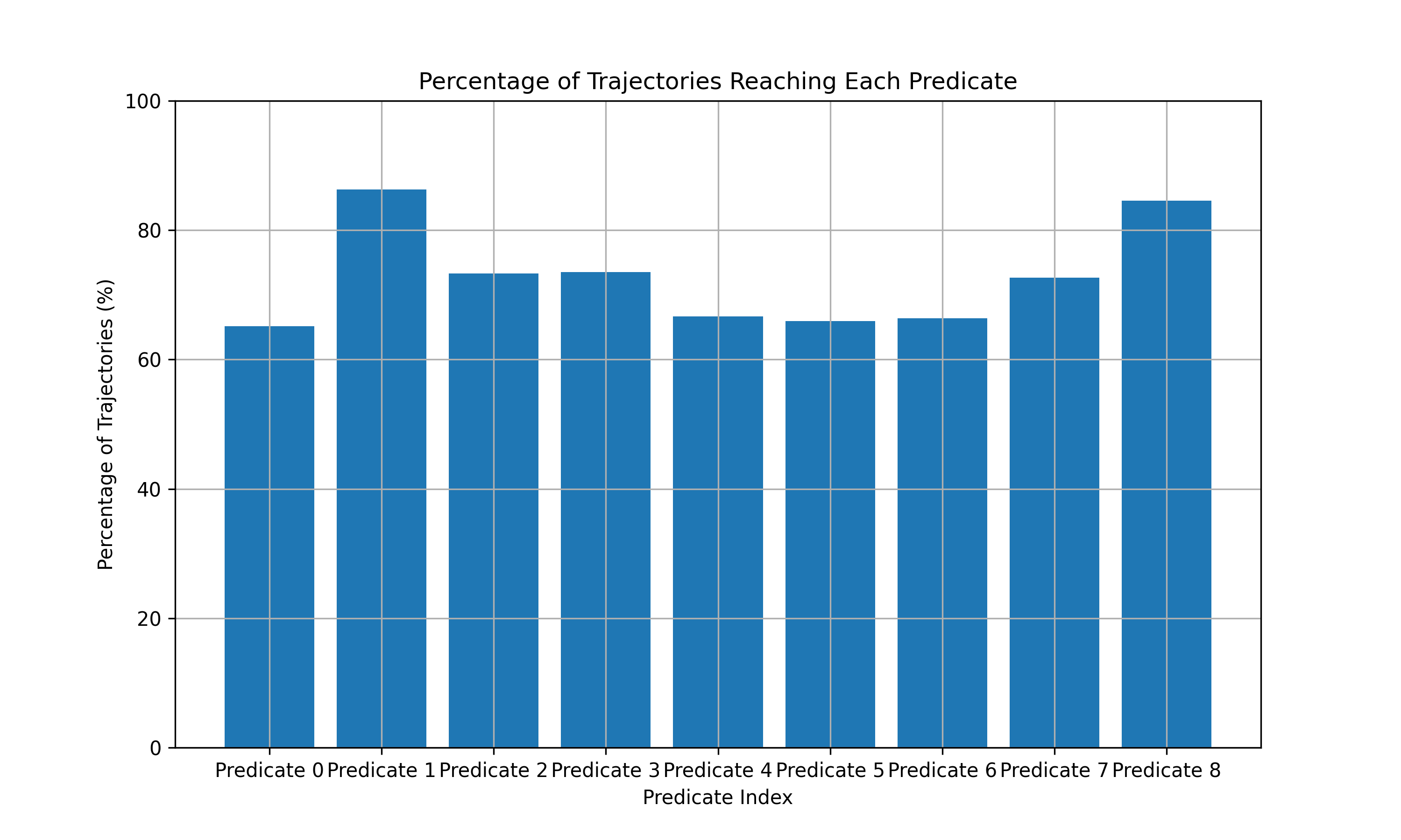
SingleIntegrator Predicate Coverage

Predicate coverage for SingleIntegrator dataset

Top: Coverage of dataset over predicates (SingleIntegrator).

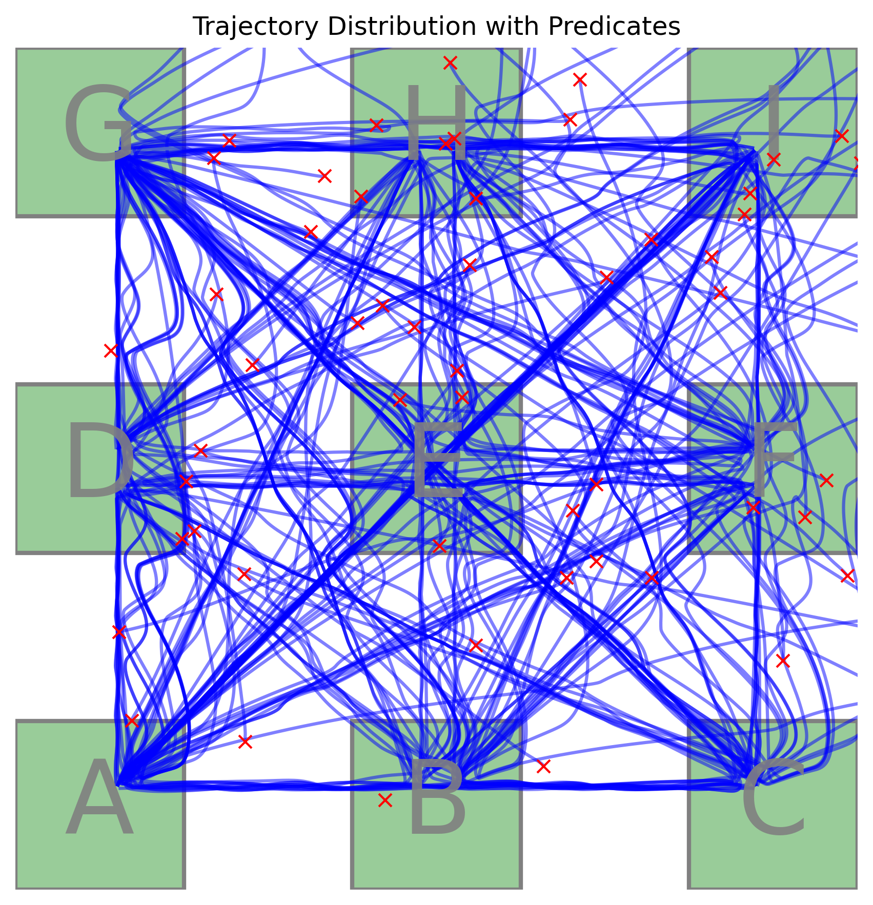
DubinsCar Trajectory Samples

Example trajectories for DubinsCar dataset

Bottom: Visualizing a subset of dataset trajectories (DubinsCar).

JIT Compilation & Resampling

JIT (XLA) compilation. We use JAX/XLA just‑in‑time compilation. The first call for a given planner/specification shape triggers a one‑time compile; subsequent evaluations reuse the compiled graph. We therefore separate this cost from the planning metrics and report it explicitly as “JIT Comp. Time (↓)”.

Resampling. Our diffusion planner may resample candidate plans if the intermediate STL loss exceeds a threshold. Each resample iteration has approximately fixed runtime cost, but the number of resamples depends on the specification and number of agents. We therefore report “Num. Resampling (↓)” alongside other metrics.

Achievable-loss ablation. We also include an ablation variant that removes the achievable loss term, denoted “D‑MA (No Ach.)”. This variant changes both compile costs (fewer STL constraints) and resampling behaviour.

Planning‑time results in the main tables exclude the one‑time JIT compile and report resampling counts separately for transparency.

Compilation and Resampling times for the Dubins Car environment in the Homogeneous task setting. D‑MA: Diffusion‑based Multi‑Agent (Ours), D‑MA (No Ach.): ablation without achievable loss, D‑SA: Diffusion‑based Single‑Agent.
Spec N JIT Comp. Time (↓) Num. Resampling (↓)
D‑MA D‑MA (No Ach.) D‑SA D‑MA D‑MA (No Ach.) D‑SA
Branch 874.2418.247.791.121.001.00
1687.8316.649.791.061.001.00
32120.4139.7812.451.061.001.47
Cover 832.2510.706.041.001.121.50
1679.9215.077.201.121.122.25
3271.0023.488.731.031.002.47
Loop 8130.0873.7722.521.881.886.38
16184.14131.9830.351.811.817.06
32287.6896.9242.363.123.066.91
Seq. 857.988.826.021.751.001.12
1643.1116.716.581.061.061.44
3282.4214.488.251.411.411.62